
Results Viewer
The Results panel loads OpenFAST binary output files (.outb), displays time-series and spectral plots, computes statistics, and enables direct comparison between multiple runs. Click Results under INSPECT in the sidebar to open it.
Loading runs
Section titled “Loading runs”Scan folder
Section titled “Scan folder”Click Scan folder (top right) to open the output file scanner.
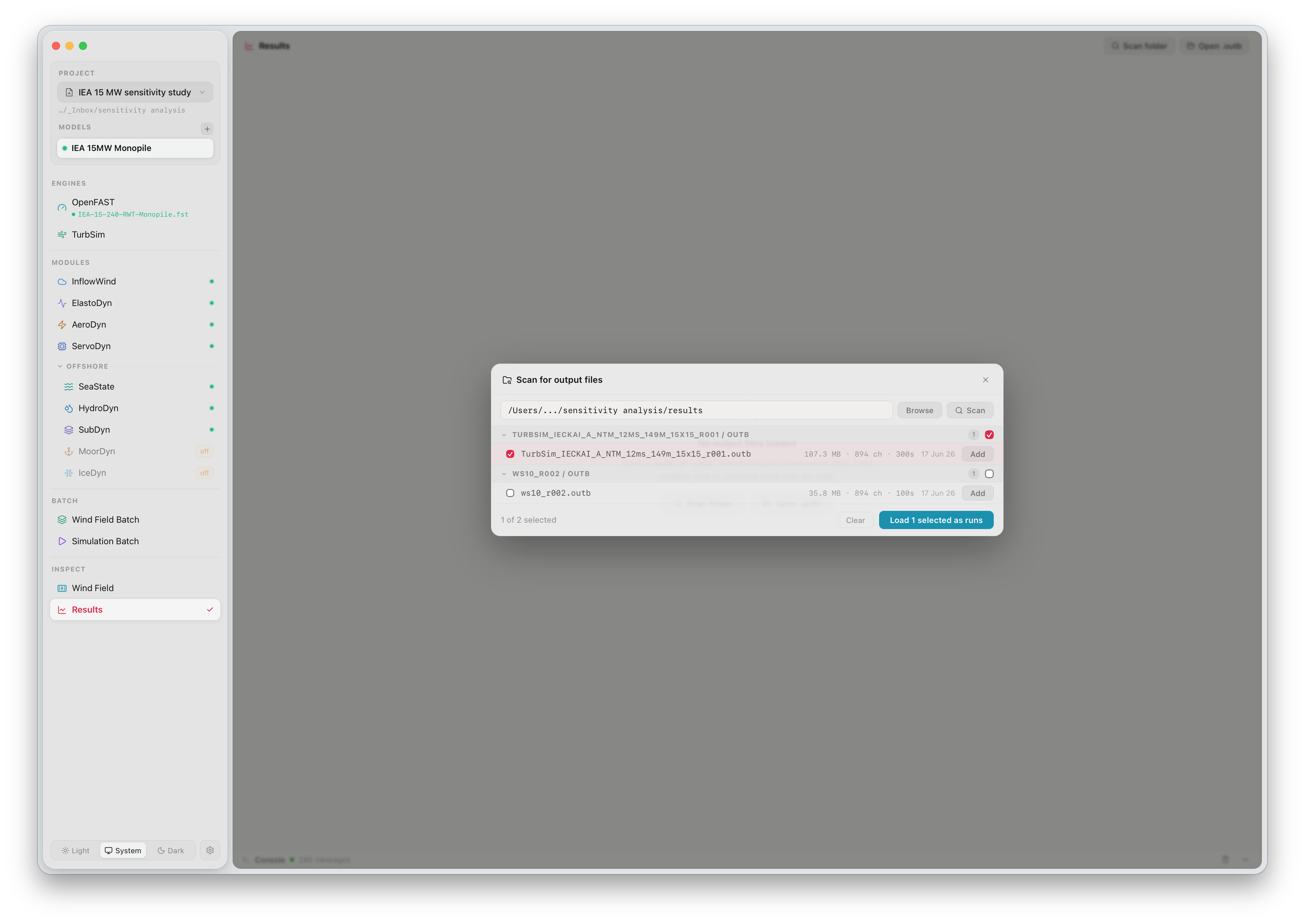
The scanner searches the specified directory recursively for .outb files. For each file found it shows:
| Column | Description |
|---|---|
| Filename | The .outb file and its containing folder |
| Size | File size in MB |
| Channels | Number of output channels in the file |
| Duration | Simulation duration in seconds |
| Date | File modification date |
Select the files you want to load using the checkboxes, then click Load selected as runs. Each loaded file becomes a run in the session.
The path field defaults to the current project’s results/ directory. Click Browse to navigate to any folder. Click Scan to refresh the file list after adding new results.
Open .outb
Section titled “Open .outb”The Open .outb button (top right) opens a single file directly from the file system — useful for loading a result from outside the current project directory.
Run tabs
Section titled “Run tabs”Each loaded run appears as a tab below the toolbar showing a shortened run name. Click a tab to bring that run to the foreground. All loaded runs remain visible simultaneously on the same plot for comparison.
Click the × on a tab to remove the run from the session. The file on disk is not affected.
Channels
Section titled “Channels”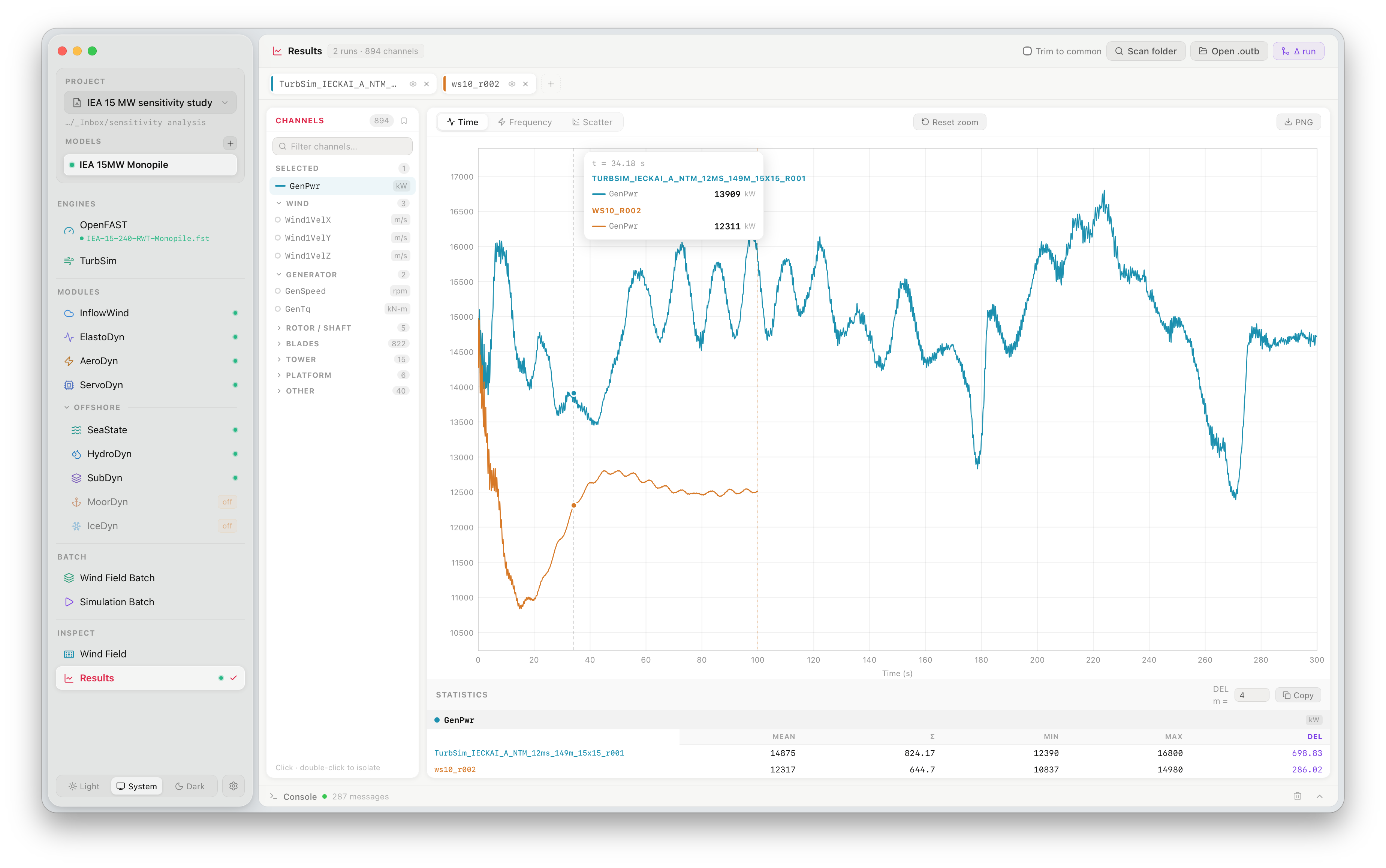
The CHANNELS panel on the left lists all output channels available in the loaded files, organised by category:
| Category | Typical channels |
|---|---|
| WIND | HorWindV, WindVxi, WindVyi |
| ROTOR / SHAFT | RotSpeed, RotTorq, RotPwr |
| GENERATOR | GenSpeed, GenTq, GenPwr |
| BLADES | BlPitchxx, RootMxx, TipDxxx |
| TOWER | TwrBsMyy, TwrBsMxt, TTDspFA |
| PLATFORM | PtfmSurge, PtfmHeave, PtfmPitch |
Click a channel name to add it to the SELECTED list and plot it. Click again to deselect. Use the search box at the top of the channel list to filter by name — useful when working with the hundreds of channels a full offshore model produces.
Plot views
Section titled “Plot views”Three plot modes are available via the tabs above the plot area.
Time series
Section titled “Time series”Plots selected channels against simulation time. All loaded runs are overlaid on the same axes using distinct colours, making run-to-run comparison immediate.
A hover crosshair snaps to the nearest data point and shows the exact value and run name in a tooltip. Use Reset zoom to return to the full time range after scrolling or zooming.
Frequency (PSD)
Section titled “Frequency (PSD)”Switches the plot to a Power Spectral Density view showing energy distribution across frequencies. Useful for identifying resonance peaks, rotor harmonics (1P, 3P), and tower natural frequencies.
Scatter
Section titled “Scatter”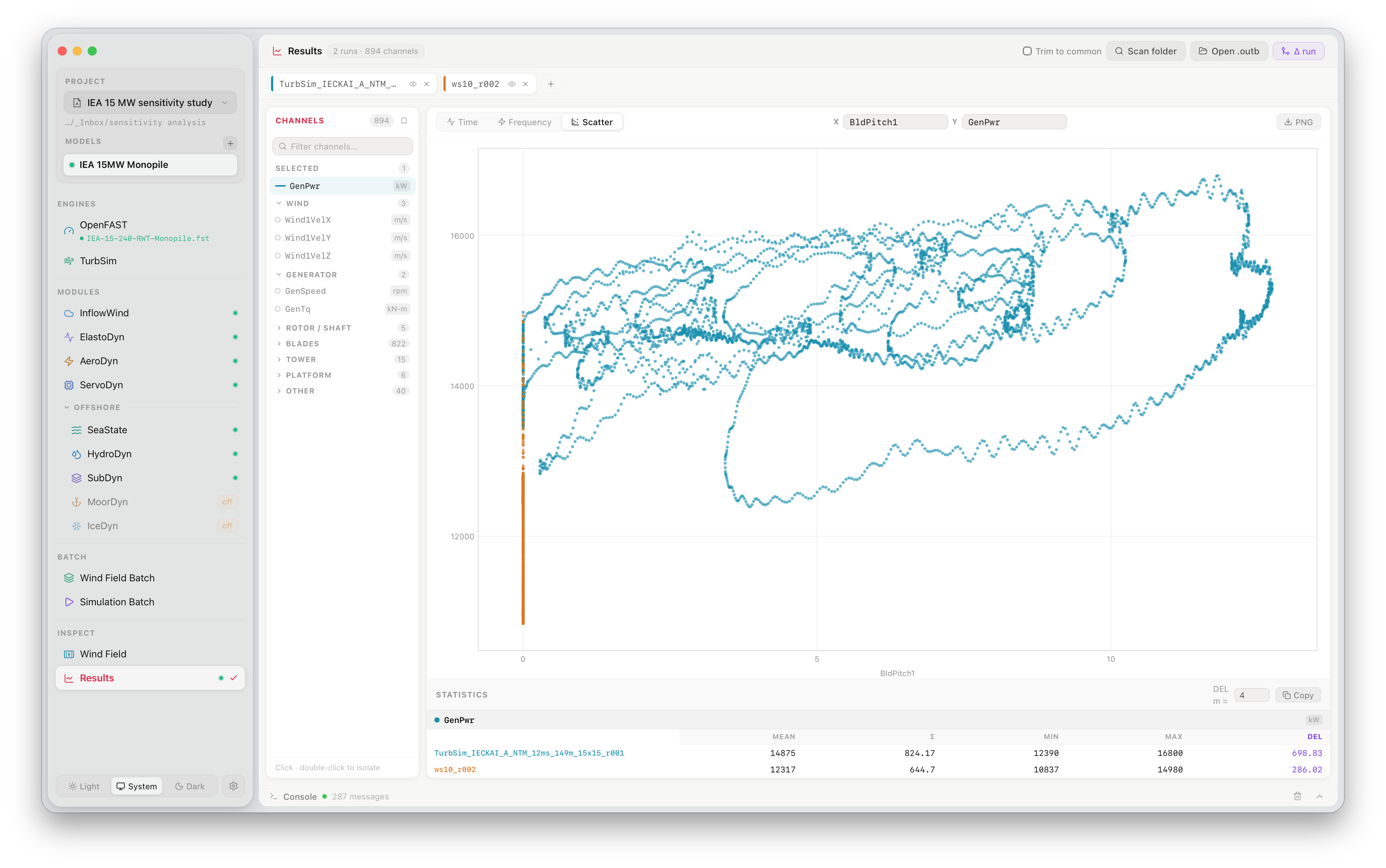
Scatter mode plots one channel against another. Select the X-axis channel using the dropdown at the top right of the plot area and the Y-axis channel from the CHANNELS panel. All loaded runs are overlaid, each in its own colour.
The scatter view is particularly useful for examining pitch–power relationships, torque–speed curves, and any other channel pair that reveals dynamic turbine behaviour.
Statistics
Section titled “Statistics”Below the plot, the STATISTICS table shows summary statistics for all selected channels across all loaded runs:
| Column | Description |
|---|---|
| Mean | Time-averaged value over the full simulation |
| Std | Standard deviation |
| Min | Minimum value |
| Max | Maximum value |
| DEL | Damage Equivalent Load, computed using the Wöhler exponent m |
The DL field (default 4) controls the Wöhler exponent used for DEL calculations. Use 4 for steel tower and monopile structures; use 10 for composite blade materials. Click Copy to copy the statistics table to the clipboard as tab-separated values.
Comparing runs
Section titled “Comparing runs”Any number of runs can be loaded simultaneously. All active runs are plotted together with distinct colours and included in the statistics table as separate rows. This makes it straightforward to compare different wind speeds, turbulence seeds, or cases from a Simulation Batch.
Exporting data
Section titled “Exporting data”Use the Copy button in the statistics panel to copy summary statistics to the clipboard. For full time-series export, use external tools such as openfast_toolbox or MATLAB’s readFASTbinary with the .outb file directly.